
Lesson 11
Bode plots and resonance
Learn to do gain and phase Bode plots for transfer functions of ω and s in the Plotting Tools card. Find the resonant frequency of an answer by solving for the frequency at which the reactance vanishes.
Last updated 2026-08-27
Two things that only make sense across a range of frequencies rather than at one: the Bode plot, which draws a transfer function's gain and phase as frequency sweeps, and resonance, which is the one frequency where a circuit's reactance vanishes.
11.1Do Bode plots
A Bode plot shows the gain and the phase of a transfer function against frequency, on a logarithmic axis.
Symbulator draws it in the Plotting Tools card below the results. Solve the circuit first, then set Plot type to Bode plot of a variable (FD); the two time boxes become frequencies.
e,1,0,1
r1,1,2,1000
c1,2,0,1e-6- Variable to plot:
v2 - Start frequency (Hz) and End frequency (Hz): 10 and 100000
- Points: 300
Both curves appear together, magnitude in decibels above and phase in degrees below. For this low-pass RC that is the rolloff you would expect: flat at low frequency, falling 20 dB per decade after the corner, with the phase heading for −90°.
When you have H(s) itself
The textbook often hands you the transfer function and no circuit. Symbulator takes it directly: set Plot type to Bode plot of a transfer function H(s) (FD), and the variable box becomes Transfer function H(s). Type the function there; the Circuit Description is ignored for this plot type, so it works on an empty page.
- Write the function in terms of
s. A textbook function of jω becomes one of s by writingswherever jω appears — a Bode plot sweeps the imaginary axis, where s is jω. - The expression takes the same shorthand a circuit value does —
^for powers, implied multiplication,1'k— and it must be numeric apart froms. A leftover symbol is refused by name. - The frequency boxes are in hertz. The examples in this lesson give their ranges in rad/s; divide by 2π for the same sweep in Hz (0.1 to 300 rad/s is about 0.016 to 48 Hz).
AS7's Example 14.3
Construct the Bode plots for the given transfer function.
Symbulator takes the expression directly: set Plot type to Bode plot of a transfer function H(s) (FD) and type the problem's function into the box, writing s wherever the textbook writes jω — no imaginary operator involved. The frequency boxes are in hertz, so the sweep of 0.1 to 300 rad/s is about 0.016 to 48 Hz.
200*s/((s+2)*(s+10))- Start frequency (Hz) and End frequency (Hz): 0.016 and 48
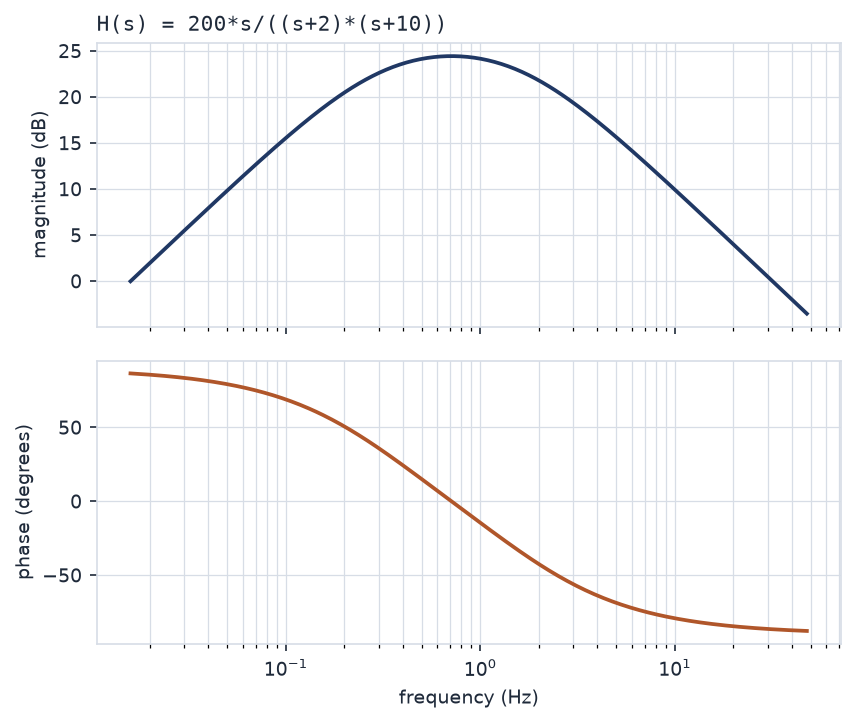
AS7's Example 14.3: the Bode plot Symbulator draws
Reading the answers off the curve: the maximum of 24.4 dB at 4.47 rad/s sits near 0.71 Hz, and the zero crossing at 199.8 rad/s near 31.8 Hz.
AS7's Practice Problem 14.3
Draw the Bode plots for the given transfer function.
The transfer-function plot type again: write the function in terms of s and sweep. The sweep of 0.1 to 100 rad/s is about 0.016 to 16 Hz.
5*(s+2)/(s*(s+10))- Start frequency (Hz) and End frequency (Hz): 0.016 and 16

AS7's Practice Problem 14.3: the Bode plot Symbulator draws
AS7's Example 14.4
Construct the Bode plots for the given transfer function.
Solved the same way: the Bode plot of a transfer function H(s) (FD) type, with the function written in terms of s.
(s+10)/(s*(s+5)^2)- Start frequency (Hz) and End frequency (Hz): 0.016 and 16

AS7's Example 14.4: the Bode plot Symbulator draws
AS7's Practice Problem 14.4
Construct the Bode plots for the given transfer function.
Symbulator always draws both, magnitude above and phase below, so there is nothing extra to ask for.
50*s/((s+4)*(s+10)^2)- Start frequency (Hz) and End frequency (Hz): 0.016 and 16
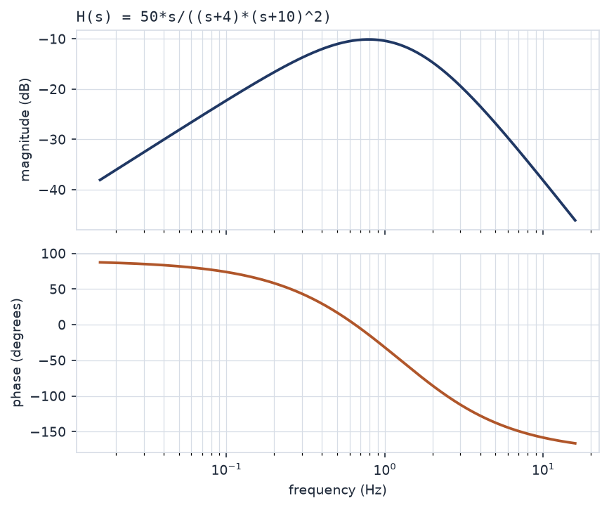
AS7's Practice Problem 14.4: the Bode plot Symbulator draws
AS7's Example 14.5
Draw the Bode plots for the given transfer function.
The same transfer-function type, and this one is already written in s. If a symbol other than s slips in, the error names it.
(s+1)/(s^2+12*s+100)- Start frequency (Hz) and End frequency (Hz): 0.016 and 16
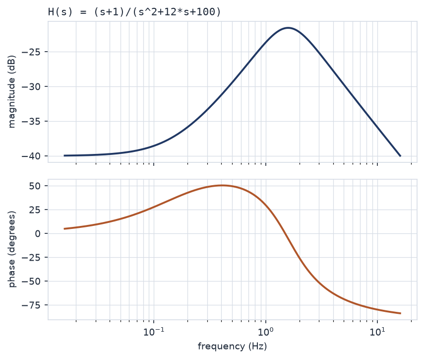
AS7's Example 14.5: the Bode plot Symbulator draws
AS7's Practice Problem 14.5
Draw the Bode plots for the given transfer function.
Nothing new here either: the transfer-function type, the function written in terms of s, both curves drawn together.
10/(s*(s^2+80*s+400))- Start frequency (Hz) and End frequency (Hz): 0.016 and 16

AS7's Practice Problem 14.5: the Bode plot Symbulator draws
11.2Resonance
The resonant frequency is the one at which a circuit's reactance vanishes — where the impedance the source sees becomes purely real.
There is no dedicated tool, and none is needed: solve the circuit in AC with w in the ω — angular frequency box, then put the condition to the Solve card.
Two things make it work, and both are easy to leave out:
- Tick real solutions only. Solving
im(ze) = 0over the complex field returns answers written in terms ofre(w)andim(w)rather thanw— useless. Declaring the unknown real is what makes it solvable. - Add
w > 0as a condition. The algebra gives ± the frequency, and only one of the two is a frequency.
AS7's Example 14.7
Open in app ↗Open in split view
Find the resonance frequency ω0 and the bandwidth frequencies ω1 and ω2.
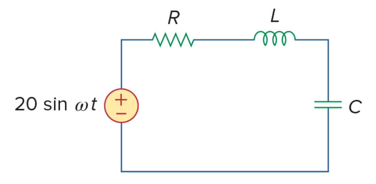
AS7's Example 14.7
Solution
e,1,0,20
r,1,2,2
l,2,3,1'm
c,3,0,.4'u
Put w in the ω box and solve in AC. Then, in the Solve card:
im(ze) = 0ww>0with real solutions only ticked. It gives ω0 = 50000 rad/s.
The bandwidth frequencies are the half-power points, where the impedance magnitude is √2 times its resistance. Same circuit, different equation:
abs(ze) = sqrt(2)*2With the condition w<50000 that gives ω1 = 49010 rad/s, and with w>50000 it gives ω2 = 51010 rad/s.
All three are correct.
AS7's Example 14.8
Open in app ↗Open in split view
Find the resonance frequency and the bandwidth frequencies.
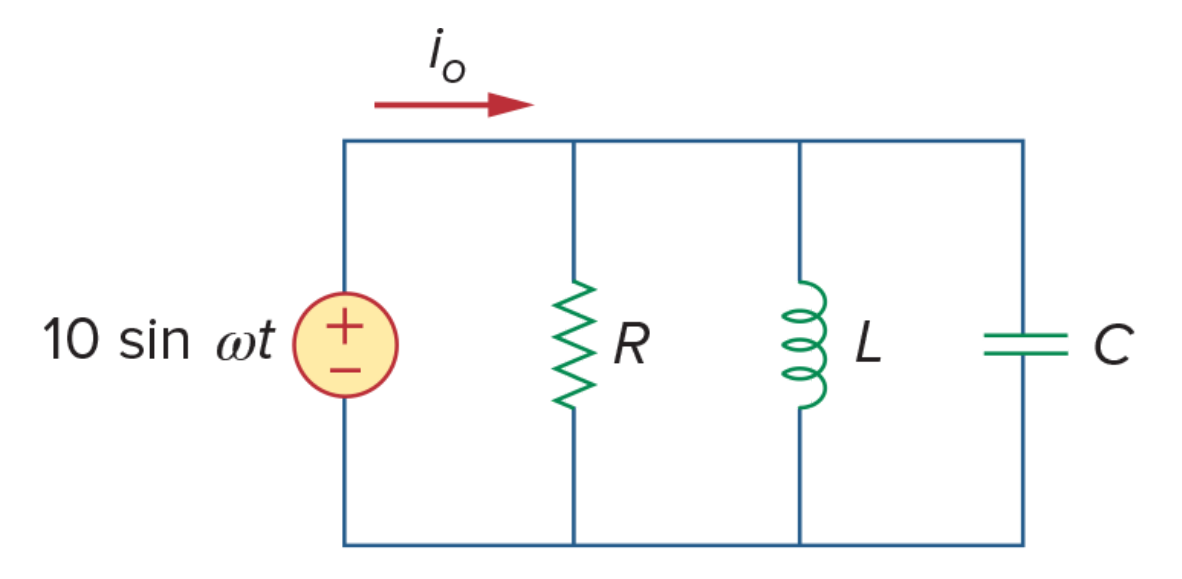
AS7's Example 14.8
Solution
e,1,0,10
r,1,0,8'k
l,1,0,.2'm
c,1,0,8'u
Trying the same equation as before does not go well here. The peak of resonance is so sharp — a needle — that a numerical search struggles to find its way to the solution. A different condition converges immediately: ask instead for the frequency at which the source's current has no imaginary part.
im(ie) = 0with w>0 and real solutions only, giving ω0 = 25000 rad/s.
Symbulator 9 solves this symbolically rather than by searching, so the sharp peak costs it nothing. The alternative equation is still worth knowing: at resonance the source sees a purely real load, so its current is in phase with its voltage.
AS7's Example 14.9
Open in app ↗Open in split view
Determine the resonant frequency ω0 of the circuit.
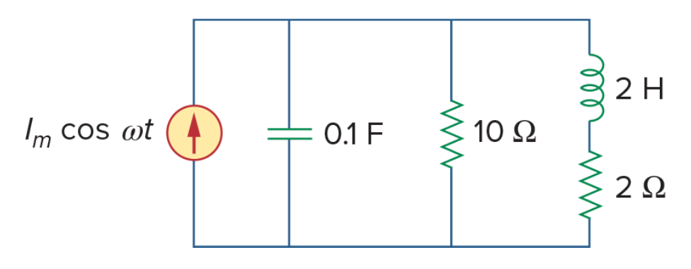
AS7's Example 14.9
Solution
j,0,1,1
c,1,0,.1
r1,1,0,10
l,1,2,2
r2,2,0,2
This time, look for the frequency at which the imaginary part of the voltage at node 1 vanishes.
im(v1) = 0with w>0 and real solutions only.
ω0 is 2 rad/s. Correct.