
Lesson 11
Bode plots and resonance
Learn to do gain and phase Bode plots for transfer functions of ω and s with the bode tool. Find the resonant frequency of an answer by solving for the frequency at which the reactance vanishes.
Last updated 2026-08-27
Two things that only make sense across a range of frequencies rather than at one: the Bode plot, which draws a transfer function's gain and phase as frequency sweeps, and resonance, which is the one frequency where a circuit's reactance vanishes.
11.1Do Bode plots
A Bode plot shows the gain and the phase of a transfer function against frequency, on a logarithmic axis.
The tool is called s\bode, and it does two kinds of plot: gain plots (also called magnitude or H(dB) plots) and phase plots. They are as good as you can expect on a TI-89.
You invoke it by entering:
s\bode()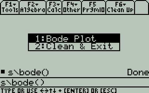
The bode tool's menu
The second option, 2: Clean & Exit, clears the variables the tool created while plotting. Use it when you are done. There is nothing more to say about it.
The first option, 1: Bode Plot, takes you to a screen with these fields:
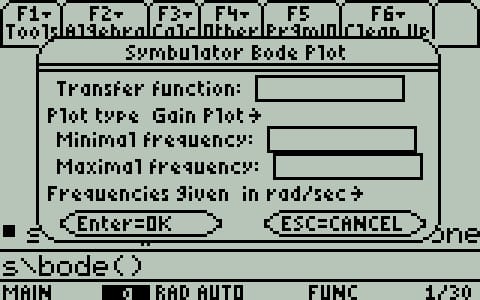
The bode tool's fields
- Transfer function — the expression you want plotted, typed directly or as the name of the variable holding it. It must be a function of a single independent variable, and that variable must be either
sorω. - Plot type — a gain plot, a phase plot, or both.
- Minimal frequency — the lowest frequency on the plot. It cannot be 0. Try 1, or 0.1, depending on the circuit.
- Maximal frequency — the highest, which must be larger than the minimum.
- The unit the two frequencies are given in.
Press Enter and Symbulator generates one or two expressions, stores them in y1(x) and y2(x), and plots them. Your independent variable has been replaced by x at that point, so every graph option — minimum, maximum, zero, trace — works normally. Just remember that x means your variable.
AS7's Example 14.3
Construct the Bode plots for the given transfer function.
We write the expression using the character the calculator understands for the imaginary operator — 𝐢, rather than the textbook's j. In my experience it pays to type it outside the tool first, where you can see it clearly:

The expression, typed outside the tool
When I'm happy with it I copy it to the clipboard, run s\bode(), and paste it into the field. Gain Plot as the type, 0.1 as the minimum frequency and 100 as the maximum, in rad/sec as the unit. Press Enter.
I wanted to see more of the plot to the right, so I pressed HOME and ran the tool again — the previous values are still there, so only the maximum needs changing. 300 gives a better-looking plot.
Press F5 and choose 4:Maximum, then pick bounds around the peak:
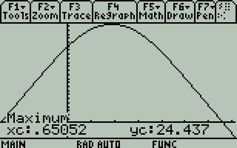
Finding the maximum
There is a maximum gain of 24.4 at x = 0.65052 — and since x is the logarithm of the frequency, that is 10^0.65052 = 4.47 rad/s.
Press F5 again and choose the zero option, with bounds around where the line crosses the axis:
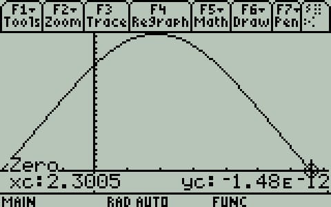
Finding the zero
That is x = 2.3005, so 10^2.3005 = 199.8 rad/s.
Now the phase plot. Run the tool again and ask for a Phase plot:
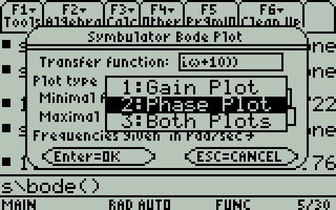
The phase plot
The Zero option works here too, and shows the phase passing through zero exactly where the gain is at its maximum:
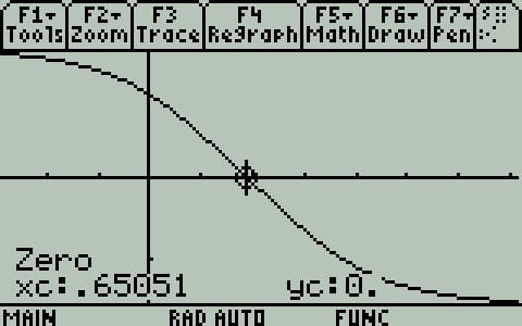
Phase zero at the gain peak
AS7's Practice Problem 14.3
Draw the Bode plots for the given transfer function.
Solved exactly as the one above. I used 0.1 and 100 as the minimum and maximum frequencies. This is the gain plot:
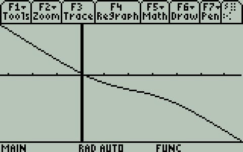
The gain plot
And this is the phase plot:
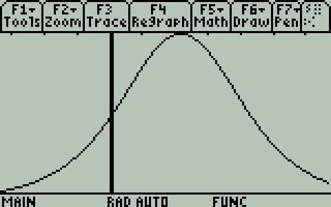
The phase plot
AS7's Example 14.4
Construct the Bode plots for the given transfer function.
Same as above. This is the gain plot:
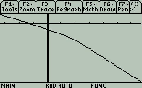
The gain plot
And this is the phase plot:
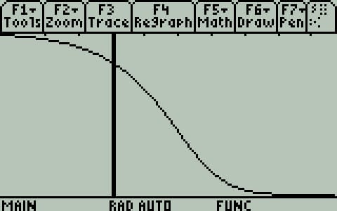
The phase plot
AS7's Practice Problem 14.4
Construct the Bode plots for the given transfer function.
Same as above, so this time let us do both plots together — the tool will draw gain and phase in one go:
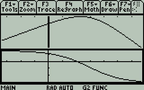
Both plots together
AS7's Example 14.5
Draw the Bode plots for the given transfer function.
To be sure of typing it clearly, write the expression outside the tool first:
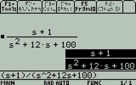
The expression
Gain Plot, 0.1 as the minimum frequency and 100 as the maximum, in rad/sec as the unit. Press Enter and we get this:
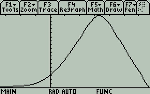
The gain plot
Now the phase. Press HOME, run the tool again, and ask for a Phase plot:
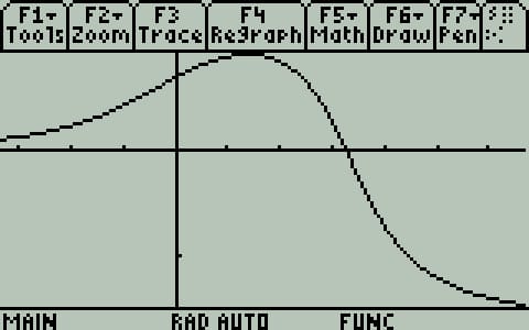
The phase plot
AS7's Practice Problem 14.5
Draw the Bode plots for the given transfer function.
Solved the same way as the one above, so there is nothing new to show. Let me use it instead to demonstrate plotting gain and phase together:
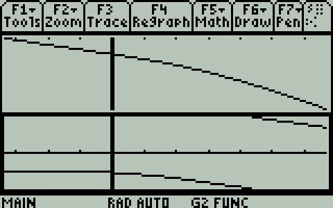
Gain and phase together
11.2Resonance
The resonant frequency is the one at which a circuit's reactance vanishes — where the impedance the source sees becomes purely real.
There is no dedicated tool. You solve the circuit symbolically in ω and then put the condition to the calculator's Numeric Solver (APPS, then 9), or to nSolve.
AS7's Example 14.7
Find the resonance frequency ω0 and the bandwidth frequencies ω1 and ω2.
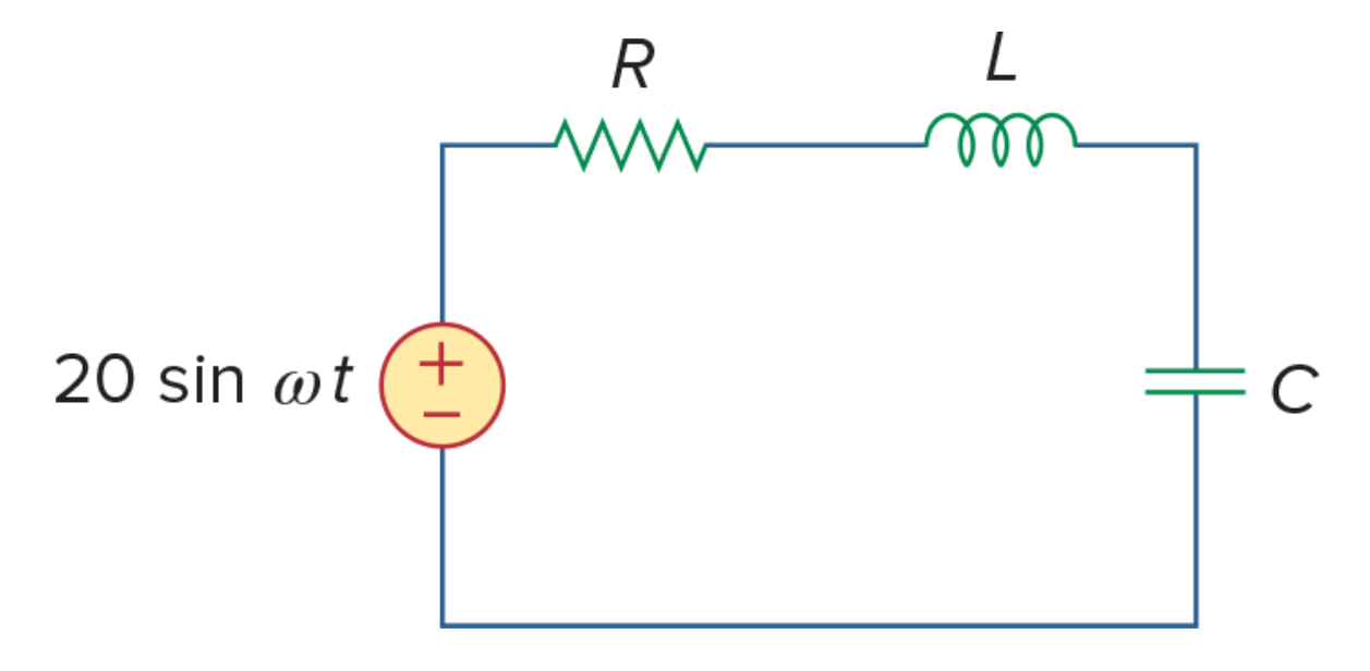
AS7's Example 14.7
Solution
"e,1,0,20.:r,1,2,2.:l,2,3,1.'m:c,3,0,.4'μ"→cir:s\ac(cir,ω)In the Numeric Solver's eqn field, enter abs(ze)=real(ze). It offers an interval for ω from −1ᴇ14 to 1ᴇ14; since there is no negative frequency here, change the lower bound to 0:
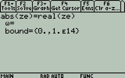
The Numeric Solver, ready
With the cursor in the blank next to ω=, press F2 Solve:
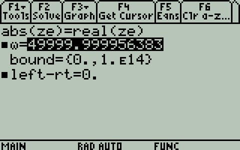
The resonant frequency
So ω0 is 50000 rad/s. For ω1, the lower bandwidth frequency, change the equation and the bounds:
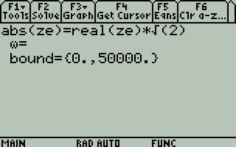
Set up for the lower bandwidth frequency
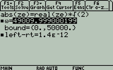
ω1
ω1 is 49010 rad/s. For the upper one, change the bounds again:
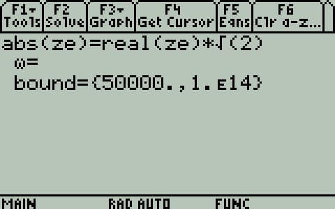
Set up for the upper bandwidth frequency
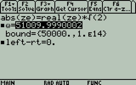
ω2
ω2 is 51010 rad/s.
All three are correct.
AS7's Example 14.8
Find the resonance frequency and the bandwidth frequencies.
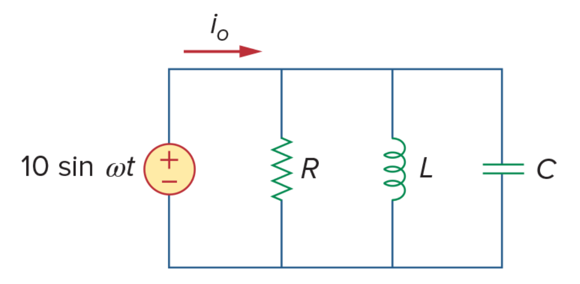
AS7's Example 14.8
Solution
"e,1,0,10:r,1,0,8'k:l,1,0,.2'm:c,1,0,8'μ"→cir:s\ac(cir,ω)Trying the same equation as before does not go well here. The peak of resonance is so sharp — a needle — that a numerical search struggles to find its way to the solution. A different condition converges immediately: ask instead for the frequency at which the source's current has no imaginary part.
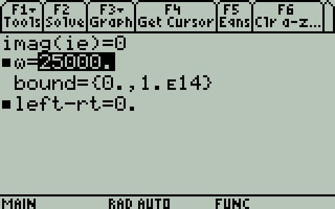
imag(ie)=0 converges at once
ω0 is 25000 rad/s. For ω1, go back to the previous example's equation and change the bounds:
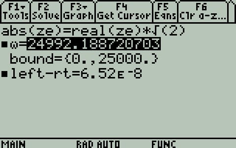
ω1
ω1 is 24992.2 rad/s. And for ω2:
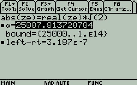
ω2
ω2 is 25007.8 rad/s.
AS7's Example 14.9
Determine the resonant frequency ω0 of the circuit.
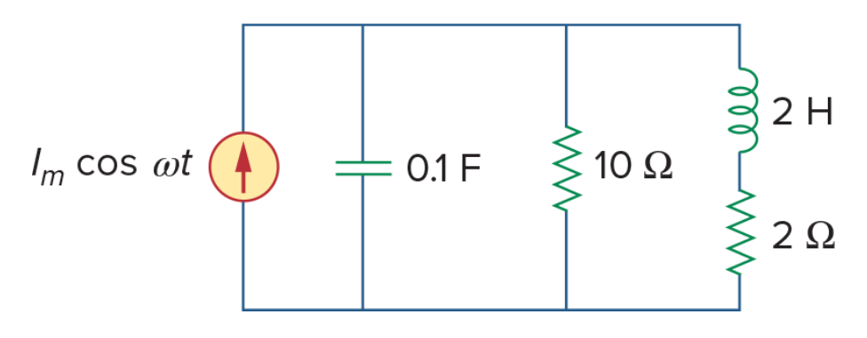
AS7's Example 14.9
Solution
"j,0,1,1:c,1,0,.1:r1,1,0,10:l,1,2,2:r2,2,0,2"→cir:s\ac(cir,ω)This time, look for the frequency at which the imaginary part of the voltage at node 1 vanishes.
nSolve(imag(v1)=0,ω)|ω>0ω0 is 2 rad/s. Correct.