
Lesson 8
Power in AC circuits
Learn to solve average power and complex power problems in AC. Learn how you can use RMS values in Symbulator with the rms flag. Solve power factor problems using the pf tool.
Last updated 2023-07-08
In this lesson you will learn how to run more advanced alternating current simulations. You will learn how to solve average power problems, when and how to use the rms flag, and how to solve complex power problems.
8.1Average power
AS7's Example 11.5
Determine the load impedance ZL that maximises the average power drawn from the circuit. What is the maximum average power?
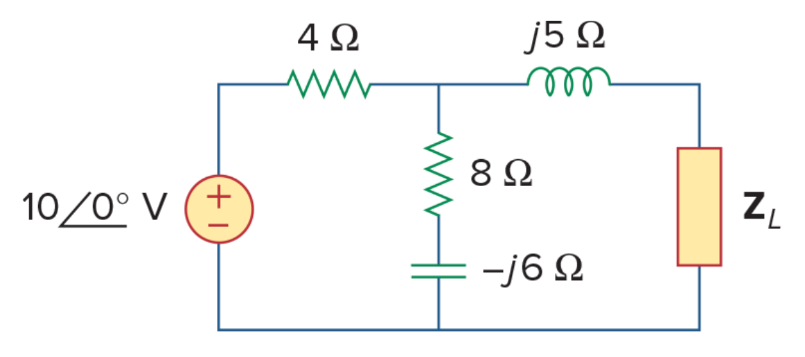
AS7's Example 11.5
Solution
Symbulator's th tool helps us find all the answers we need. Notice this circuit description does not include the load, because it is not needed as input to th.
"e,1,0,10:r1,1,2,4:r2,2,0,8-6𝐢:r3,2,3,5𝐢"→cir
s\th(cir,3,0)
When asked a type of analysis, specify AC. Then you will be asked if a load problem is next. You don't have to answer Yes, but I invite you to, because I want to show you something cool.
The s\th tool saves the equivalent impedance in zeq, which evaluates approximately to 2.933 + j4.467. The load that will deliver the maximum power is its conjugate, 2.933 − j4.467.
The average maximum power delivered by the circuit is in apmax, which evaluates to 2.3674 W.
Now, here's the cool part: when you answer Yes to the load question, Symbulator saves expressions for the current through, voltage drop in, average power and complex power in a load connected to the equivalent circuit, as a function of the complex value of that load — the variable load_, where the underscore tells the calculator to treat this variable as complex. This means you can verify that this is the maximum power delivered:
aprl|load_=conj(zeq)It evaluates to the same answer.
2.36742424242424It is the same answer.
8.2RMS and PF
In the previous lesson we mentioned that after an AC simulation you also get the complex power consumed. How to read these values depends on a flag called the RMS flag.
The s\rms flag
You will learn in your circuits course that phasor analysis can be done in RMS values. There are advantages to it, and you will have to solve AC circuits both in normal values (also called magnitude values) and in RMS. Working in RMS simply means every current and voltage in the analysis is taken to be RMS. That's it.
The flag that tells the program which you want is stored in a variable called s\rms, and it can be true or false. By default, it is false.
When the flag is false, AC analysis assumes normal values: Symbulator assumes all the currents and voltages you give it are magnitude values, gives you all the answers in magnitude values, and stores the average real power consumed in r, e, j and o elements in a variable called ap plus the element name.
When the flag is true, AC analysis assumes RMS values throughout, and the average real power consumed lands in a variable called p plus the element name.
AS7's Example 11.10
Determine the power factor of the entire circuit as seen by the source. Calculate the average power delivered by the source.
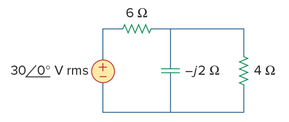
AS7's Example 11.10
Solution
The source value in this problem is given in RMS values, so we must say so.
true→s\rms
"e,1,0,30.:r1,1,2,6.:r2,2,0,-𝐢2.:r3,2,0,4."→cir
s\ac(cir,ω)
Or, if you want to simplify the impedances, the resistors can be collapsed into a single parallel combination.
The average power consumed by the source is in pe. To get the average power delivered, we ask for the negative of it, which gives us 125.4 W.
The pf tool
To find the power factor of an element answer, we can use the s\pf tool. We can use this tool in two ways.
With a complex expression as input. One way is to give it a complex expression, with real and imaginary parts. It can contain symbolic and/or numerical values, exact or approximate; it can be a complex number in rectangular or angular form; or it can be a variable holding such an expression, such as the complex power consumed in an element:
s\pf(se)The pf tool takes this complex value and calculates the power factor as the absolute value of the real part divided by the magnitude of the whole thing.
Now, this is not the whole picture: we need to know whether this power factor is leading or lagging.
With an element name as input. The second way is to give it a string with the name of a single element that was part of an s\ac simulation that just finished. The tool recognises three elements in this form: e, j and r:
s\pf("e")pf: 0.97342 leadingIn a nutshell: given a complex number or expression, pf returns the power factor but says nothing about leading or lagging. Given the name of an element in a string, right after an s\ac simulation, it returns the value and says which. That second form works only if the expression can be evaluated numerically.
8.3Complex power
AS7's Example 11.13
The figure shows a load being fed by a voltage source through a transmission line. The impedance of the line is represented by the (4+j2) Ω impedance and a return path. Find the real power and reactive power delivered by the source, and absorbed by the line and load.

AS7's Example 11.13
Solution
The value of this circuit's source is given in RMS. Since the problem asks for answers regarding the line and the load, we should have separate impedances, one for each.
true→s\rms
"e1,1,0,220.:r1,1,2,4.+2.𝐢:r2,2,0,15.–10.𝐢"→cir
s\ac(cir,ω)
The complex power absorbed in the source, line and load are in -se1, sr1 and sr2:
{-se1,sr1,sr2}{2163.8–911.1𝐢, 455.5+227.8𝐢, 1708.2–1138.8𝐢}These are correct.
AS7's Practice Problem 11.10
Calculate the power factor of the entire circuit as seen by the source. What is the average power supplied by the source?
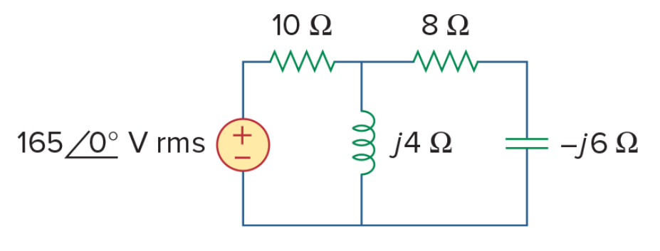
AS7's Practice Problem 11.10
Solution
The values are RMS, so set true→s\rms.
true→s\rms:"e,1,0,165.:r,1,0,10.+[𝐢4.,8.-𝐢6.]"→cir:s\ac(cir,ω)-pe gives 2007.1 W; s\pf("e") gives pf: 0.93595 laggingAS7's Problem 11.97
A power transmission system is modelled as shown. If Vs = 240 V rms, find the average power absorbed by the load.
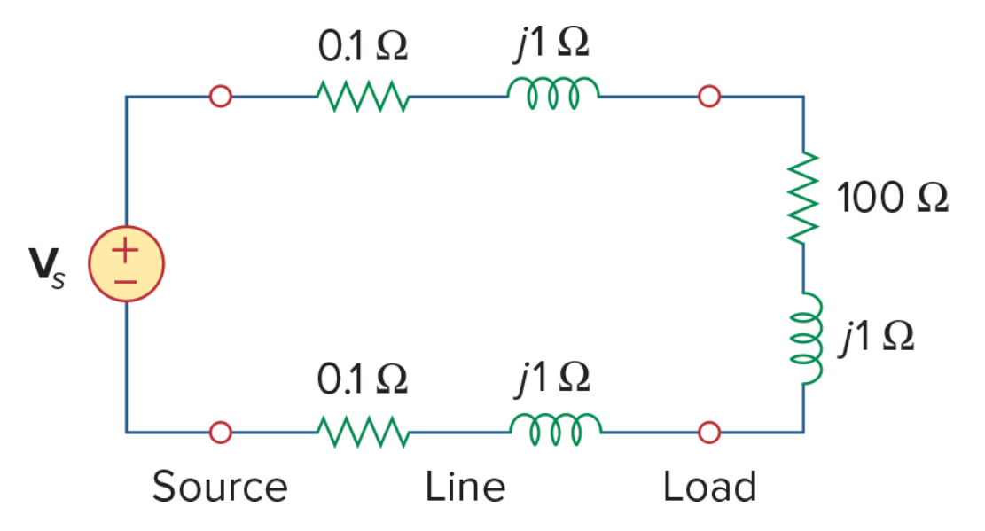
AS7's Problem 11.97
Solution
Three impedances in series: the outgoing line, the load, and the return path.
true→s\rms:"evs,1,0,240.:rl1,1,2,.1+𝐢:rl,2,3,100+𝐢:rl2,3,0,.1+𝐢"→cir:s\ac(cir,ω):prl573.2 WCorrect.
AS7's Problem 11.75
Consider the power system shown. Calculate the total complex power, the power factor, and the parallel capacitance needed for a unity power factor.

AS7's Problem 11.75
Solution
Three loads in parallel across a 240 V rms source. The first two parts need no frequency at all, so leave omega as anything.
true→s\rms:"e,1,0,240:r1,1,0,80-𝐢50:r2,1,0,120+𝐢70:r3,1,0,60+𝐢0"→cir:s\ac(cir,ω)(a) The complex power delivered is the opposite of the power the source consumes: -se gives 1835.9 − 114.7j VA.
(b) The power factor, from s\pf("e"), is 0.99805 leading.
(c) This one needs a frequency, because it needs a capacitor. Add one in parallel with a symbolic value (let's say x), and run at the stated 50 Hz — (2π)(50) in rad/s.
"e,1,0,240:r1,1,0,80-𝐢50:r2,1,0,120+𝐢70:r3,1,0,60+𝐢0:c,1,0,x"→cir
s\ac(cir,2π50.)
solve(s\pf(se)=1.,x)-6.3 μFA negative capacitance, and no positive value satisfies the equation — which is probably why the textbook gives no number for this part. It is not a failure of the method: the load is already leading, as part (b) said, so no capacitor can bring it to unity. What it needs is the opposite.
Try an inductor instead:
"e,1,0,240:r1,1,0,80-𝐢50:r2,1,0,120+𝐢70:r3,1,0,60+𝐢0:l,1,0,x"→cir
s\ac(cir,2π50.)
solve(s\pf(se)=1.,x)1.5987 HCheck it by putting that number back in as the inductor's value: the power factor comes out 1. An inductor of about 1.6 H in parallel is what brings this system to unity.