
Lesson 6
Transient analysis
Learn to run a transient time-domain analysis with tr. Learn to describe capacitors with c and inductors with l. Save time with the only tool. Plot expressions in time with the plot tool.
Last updated 2026-08-29
Symbulator can simulate two energy-storing elements, capacitors and inductors, in three kinds of analysis: transient time-domain (TR), alternating current (AC), and complex frequency-domain (FD). This lesson teaches the transient analysis of a circuit, and how to describe capacitors and inductors for it. AC and FD come in later lessons.
6.1How to describe a capacitor
Values can use SI prefixes
The values of the capacitance and the initial condition of the capacitor can use prefixes of the International System.
What answers do you get
For each capacitor, a transient analysis will provide two answers: the voltage drop in the capacitor, in volts, and the current through it, flowing from the first node towards the second, in amperes.
6.2How to describe an inductor
For each inductor, a transient analysis will provide the voltage drop across it and the current through it, with the same conventions as for capacitors.
6.3Running a transient analysis
You will learn the subtleties of transient simulations through a series of examples. For now, to run one we use an access program called s\tr, which takes one argument: the circuit description in string form.
For transient simulations, Symbulator uses the Laplace Functions by Lars Frederiksen. Make sure you have them properly installed!
Bo2's Example 4.15
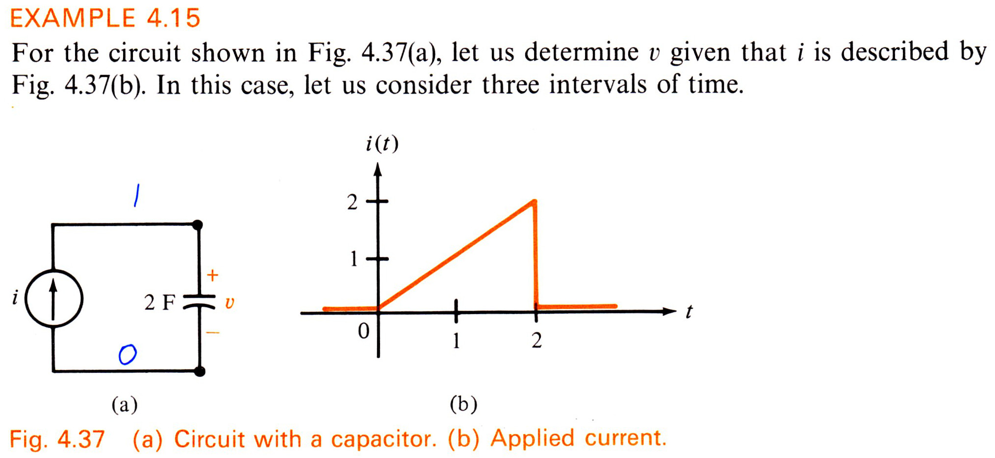
Bo2's Example 4.15
Solution
For t ≤ 0 s, since the current source is inactive, there is nothing going on. Without doing a simulation, we know the voltage v is 0 volts.
For 0 s < t ≤ 2 s, the source is active. From the graph, its value in this interval is t: the current in amperes equals the time in seconds. We describe the circuit and run the transient analysis:
s\tr("j,0,1,t:c,1,0,2,0")The source has four terms: name (starting with j), first node, second node, and value — here t. The capacitor has five: name, first node, second node, value in farads, and initial condition in volts — here 0 volts.
Once the simulation is complete, ask for the value of the voltage, vc. We get this value, which is correct:
t^2/4For 2 s < t, the voltage is equal to whatever value it had at time 2 s:
vc|t=2We get a value of 1 volt, which is correct.
Describing source values
For the purpose of a transient analysis, Symbulator accepts many types of source values. The only thing you must do is describe these values properly.
Step values: symbolic. A source with an unknown step value starting at t=0 is described with a variable and the step function u(t). For example, a voltage source e1 between nodes 1 and 0, of V volts starting at t=0, is e1,1,0,V*u(t).
Step values: numerical. A step source with a known numerical value can be described the same way, e1,1,0,12*u(t). To save typing, you can skip the u(t) when the value is numerical, and Symbulator assumes a step: e1,1,0,12. The results are the same.
Impulse values. A source with an impulse value at t=0 is described with its value, symbolic or numerical, and the delta function δ(t). For example, a current source j1 between nodes 0 and 1, with an impulse of i amperes at t=0, is j1,0,1,i*δ(t).
Values as functions of time. A source whose value is a function of time, such as a ramp, a sinusoid or an exponential, is described by writing the value as an expression in terms of t, as in j,0,1,t. Values as functions of t will activate the Impala mode, in order to save time.
Dependent values. Sources with dependent values are described as we have seen before, for example j,0,1,3*vr1.
A word on intervals
In a transient analysis, every switch opening or closing ends one time interval and begins another, and a simulation covers one interval only. When we run a TR simulation and get answers in terms of t, this variable must be understood as the time elapsed since the start of that interval in particular.
This is a distinction without a difference as long as the interval we simulate starts at t=0, which is most often the case. However, sometimes problems have switch changes at other times — Bo2's Example 5.6, where a switch closes at t=1 s, and Bo2's Drill Exercise 5.6, where one closes at t=2 s, are examples in the solved problems.
6.4Two useful tools
The only tool
Unless you say otherwise, a Symbulator simulation gives you the whole set of answers: voltages in all nodes, and voltage drops, currents and power consumed in all elements. When the expressions are complicated, storing them all takes time.
In case you don't want all the answers, but only a chosen few, you may save some time by using the s\only tool to tell Symbulator — before the simulation — which answers you want to save. Find it in Symbulator's custom menu. Its argument is either an empty variable or a string with a variable or a list of variables separated by commas. All of these are valid:
s\only(ir1)
s\only("ir1")
s\only("ir1,va,vr2")
The s\only tool is valuable in TR analysis: you save time by not having Symbulator find the inverse Laplace of answers you do not need.
The plot tool
Very often we are asked to plot functions of time. The calculator has extensive plotting capabilities, but just to save you some time, Symbulator includes a handy s\plot tool that allows you to plot functions of time.
s\plot()6.5Instructive solved examples
Transient analysis of RC circuit
Bo2's Example 5.1

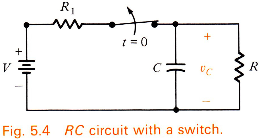
Solution. Here we have two intervals. In the first, t < 0s, we assume things have been steady for a long time and any transient has passed, so we run a DC simulation to find the initial conditions for the second.
s\dc("e,1,0,V:r1,1,2,r1:c,2,0,c:r,2,0,r")When the simulation is Done, we ask for vc, the voltage in the capacitor c. We get the expression shown below, which is correct.
For the second interval, when 0s ≤ t, we do a transient simulation. We give the capacitor as initial condition its voltage from the previous interval.
s\tr("c,2,0,c,r*v/(r+r1):r,2,0,r")When the simulation is Done, we ask for vc again. We get the expression below, which is correct.
Bo2's Drill Exercise 5.1

Solution. Again, we have two intervals: the first for DC, the second for TR.
For the first interval, when t < 0s, the current source is 2A. Simulate in DC.
s\dc("j,0,1,2:r,1,0,3:c,1,0,1/12"):{vc,ic}{ 6 , 0 }So the voltage in the capacitor is 6V. We store this value in a variable called vc0, to use it as initial condition of the capacitor for the second interval.
vc→vc0For the second interval, when 0s ≤ t, we do a transient simulation. The current source is 0A, and the capacitor has an initial condition: voltage vc0.
s\tr("j,0,1,0:r,1,0,3:c,1,0,1/12,vc0"):{vc,ic}When the simulation is Done, we get the expressions below. They are right.
Bo2's p224 5.2

Solution. Again, we have two intervals: the first for DC, the second for TR.
For the interval when t < 0s, the voltage source is 12 V. Simulate in DC.
s\dc("e,1,0,12:r3,1,2,3:r6,2,0,6:r4,2,3,4:c,3,0,1/12"):{vc,ic,v2}{ 8 , 0 , 8 }For the interval when 0s ≤ t, the voltage source is 0V. Simulate in TR, giving the capacitor as initial condition its voltage from the previous interval.
s\tr("e,1,0,0:r3,1,2,3:r6,2,0,6:r4,2,3,4:c,3,0,1/12,8"):{vc,ic,v2}Bo2's Drill Exercise 5.2
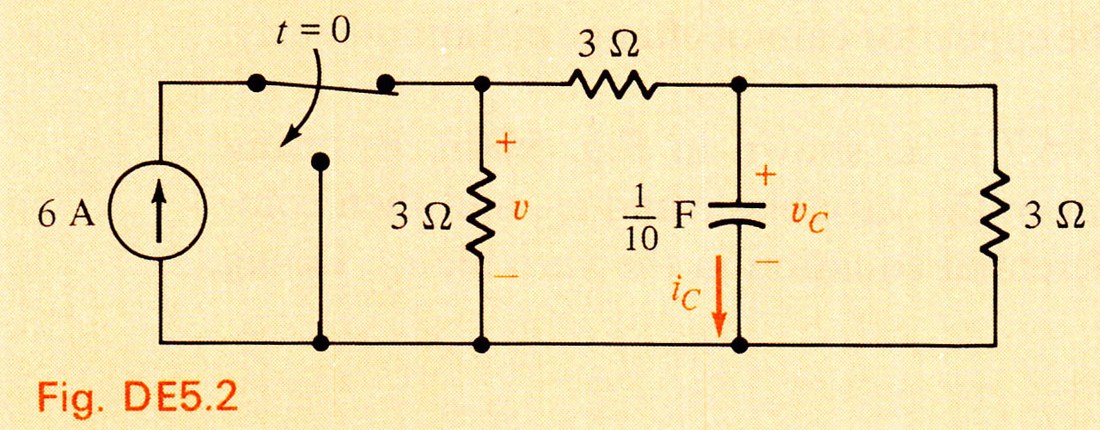

Solution. For t < 0s, the 6A source is part of the circuit. Simulate in DC.
s\dc("j,0,1,6:r10,1,0,3:r12,1,2,3:r20,2,0,3:c,2,0,1/10"):{vc,ic,v1}{ 6 , 0 , 12 }For 0s ≤ t, the source is no longer relevant and can be excluded from the circuit. Simulate in TR, giving the capacitor its proper initial condition.
s\tr("r10,1,0,3:r12,1,2,3:r20,2,0,3:c,2,0,1/10,6"):{vc,ic,v1}Bo2's Figure 5.10a
Look at the simple resistor-inductor (RL) circuit shown, where at time t=0 the inductor current is iL(0). Determine vL(t), iL(t) and vR(t) for t≥0.
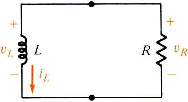
Since we are already given the initial condition, we only run the transient simulation for t≥0. In our circuit description below, the initial condition is il0.
s\tr("l,1,0,l,il0:r,1,0,r"):{vl,il,vr}We get the right answers:
Bo2's Example 5.3
Determine iL(t) for all t.
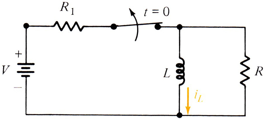
Solution. For t < 0s, simulate in DC.
s\dc("e,1,0,v:r1,1,2,r1:l,2,0,l:r2,2,0,r"):ilFor t ≥ 0s, simulate in TR, giving the inductor its initial condition.
s\tr("l,2,0,l,v/r1:r2,2,0,r"):ilBo2's Drill Exercise 5.3
Find iL(t), vL(t) and i(t) for all t.

Solution. For t < 0s, simulate in DC.
s\dc("e,1,0,8:r4,1,2,4:l,2,0,1:r12,2,0,12"):{il,vl,ir4}{ 2 , 0 , 2 }For t ≥ 0s, simulate in TR, giving the inductor its initial condition of 2A.
s\tr("e,1,0,0:r4,1,2,4:l,2,0,1,2:r12,2,0,12"):{il,vl,ir4}In my machine the simulation took 30 seconds, 12 seconds of these (40%) were used in finding the inverse Laplace of the answers — time that the only tool, described above, can save.
Bo2's p230 (Dependent source)
Find iL(t) for t≥0, given that iL(0) = 5A.

We only run the transient simulation for t≥0, with initial condition 5A.
s\tr("r,v,0,r:j,v,0,2ir:l,v,0,l,5"):ilBo2's Drill Exercise 5.4 (Dependent source)
Find iL(t) and vL(t) for all t.

Solution. For t < 0s, simulate in DC. This gives us the initial condition.
s\dc("ei,1,0,12:r6,1,2,6:l,2,0,16:r8,2,3,8:ed,3,0,3vr8"):{il,vl}{ 2 , 0 }For t ≥ 0s, simulate in TR, giving the inductor its initial condition.
s\tr("l,2,0,16,2:r8,2,3,8:ed,3,0,3vr8"):{il,vl}Bo2's Example 5.5 (Op Amp)
Determine vC(t), iC(t) and vo(t) for all t.

Solution. For t < 0s, simulate in DC. This gives us the initial condition.
s\dc("e,3,0,4:r2,3,1,2:r5,1,o,5:c,1,o,1/20:o,0,1,o"):{vc,ic,vo}{ 10 , 0 , -10 }For t ≥ 0s, simulate in TR, giving the capacitor its initial condition.
s\tr("r2,0,1,2:r5,1,o,5:c,1,o,1/20,10:o,0,1,o"):{vc,ic,vo}Bo2's Drill Exercise 5.5 (Op Amp)
Determine vC(t), iC(t) and vo(t) for all t.

Solution. For t < 0s, simulate in DC. This gives us the initial condition.
s\dc("e,2,0,4:o,2,1,o:c,o,1,1/20:r5,o,1,5:r2,1,0,2"):{vc,ic,vo}{ 10 , 0 , 14 }For t ≥ 0s, simulate in TR, giving the capacitor its initial condition.
s\tr("o,0,1,o:c,o,1,1/20,10:r5,o,1,5:r2,1,0,2"):{vc,ic,vo}Bo2's Example 5.6
In the circuit shown, there are two switches: one that opens at time t=0 and one that closes at time t=1 second. Determine vC(t) and iC(t) for all t.
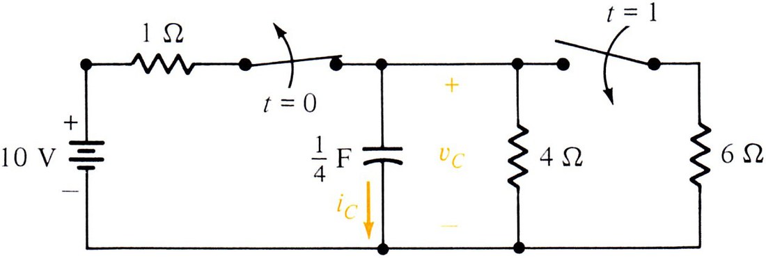
As we mentioned before, every time a switch moves marks the end of one interval and the beginning of another interval for Symbulator.
For the first interval, which corresponds to t<0, we simulate in DC.
s\dc("e,2,0,10:r1,2,1,1:c,1,0,1/4:r4,1,0,4"):{vc,ic}{ 8 , 0 }The voltage in the capacitor at the end of this interval will serve as the initial condition of the capacitor for the next interval. The second interval runs between 0 and 1 second, i.e. 0 < t ≤ 1 second. We simulate in TR.
s\tr("c,1,0,1/4,8:r4,1,0,4"):{vc,ic}The capacitor's voltage at the end of this second interval is the initial condition for the third. We can use its exact value, 8*e^–1, but the textbook prefers using its approximate value, i.e. 2.943.
The third interval corresponds to t > 1 second. We simulate in TR. To make things easier for Symbulator, we replace the resistors by their equivalent.
s\tr("c,1,0,1/4,2.943:re,1,0,[4,6]")Ask for {vc,ic}. The expressions we get are equivalent to:
These are the right answers, as can be seen by checking the book's answers.


Bo2's Drill Exercise 5.6
Let’s see another example where a TR simulation is done for an interval that starts at a time other than t=0. Determine iL(t) and vL(t) for all t.
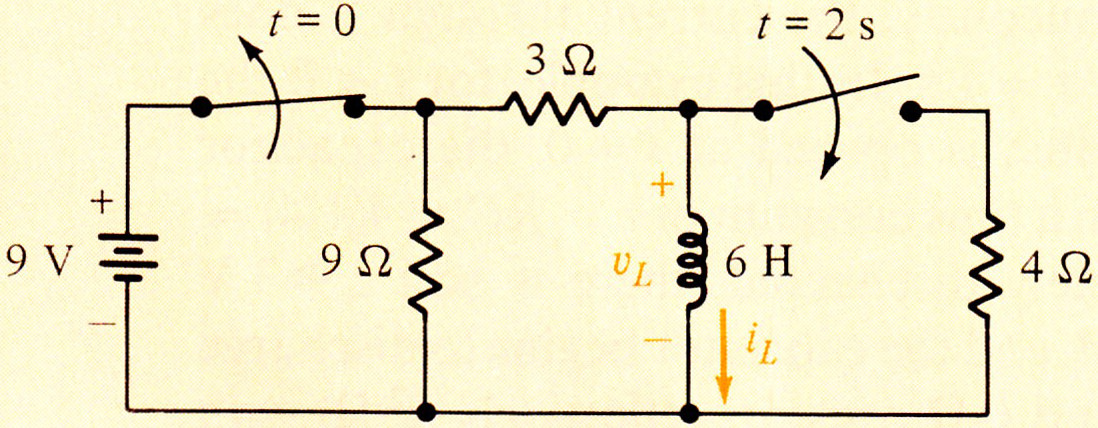
For the first interval, which corresponds to t<0, we simulate in DC.
s\dc("e,1,0,9:r9,1,0,9:r3,1,2,3:l,2,0,6"):{il,vl}{ 3 , 0 }The 3A current in the inductor is its initial condition for the second interval, which goes from 0 to 2 seconds, i.e. 0 < t ≤ 2 seconds. We simulate in TR.
s\tr("r,1,0,9+3:l,1,0,6,3"):{il,vl}The inductor's current at the end of this second interval is the initial condition for the third. Find its approximate value thus:
iL|t=2..055
The third interval corresponds to t > 2 second. We simulate in TR. To make things easier for Symbulator, we replace the resistors by their equivalent.
s\tr("r,1,0,[9+3,4]:l,1,0,6,.055"):{il,vl}These are the kind of expressions your book or professor are looking for.
Bo2's Figure 5.19
In the following circuit, assume that all the initial conditions are zero. The source is a step function u(t) with value V volts. Find iR, vR, iC and vC.

As discussed before, a step source with symbolic value requires that we use the u(t) nomenclature to describe it. Since the value is V volts, we describe the source as V*u(t).
s\tr("e,1,0,V*u(t):r,1,2,r:c,2,0,c,0"):{vc,vr,ic}There is no need to ask for iR, since iR=iC. We get the following expressions:
Bo2's Figure 5.24
In the following circuit, assume that all the initial conditions are zero. The source is a step function u(t) with value V volts. Find iR, vR, iL and vL.
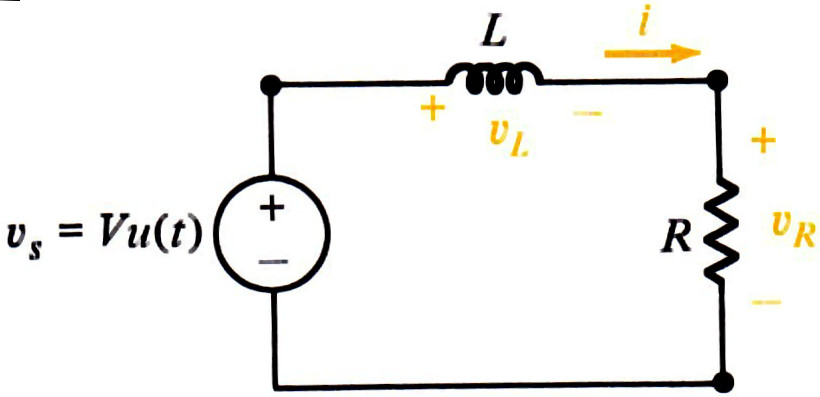
s\tr("e,1,0,V*u(t):l,1,2,l,0:r,2,0,r"):{vl,vr,il}There is no need to ask for iR, since in a series circuit it will be identical to iL.
Bo2's Drill Exercise 5.7
For the circuit, with a step source of 12 volts, find iL, vL, iL and v.
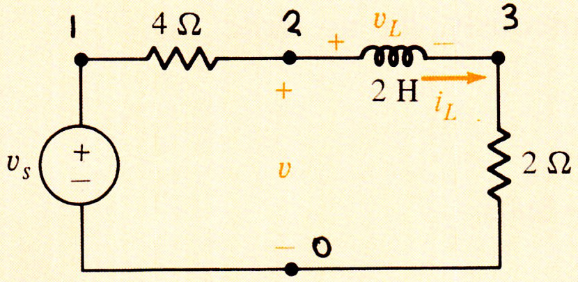
As discussed before, a step source with numerical value can be described without the u(t) nomenclature. Thus, we describe the source as 12.
s\tr("e,1,0,12:r4,1,2,4:l,2,3,2,0:r2,3,0,2"):{il,vl,v2}Bo2's Figure 5.26
In the following circuit, assume that all the initial conditions are zero. The source is a step function u(t) with value I amperes. Find iC, iR, and v.

As discussed before, a step source with symbolic value requires that we use the u(t) nomenclature to describe it. Since the value is I amperes, we describe the source as I*u(t). Thus:
s\tr("j,0,1,i*u(t):c,1,0,c,0:r,1,0,r"):{v1,ir,ic}Bo2's Example 5.7 (Op Amp)
Suppose that vs(t)=u(t). Find vC, iC, and vo.

This source is a step source with a value of 1 volt. Since its value is numerical, the u(t) nomenclature is not needed. We describe the source plainly as 1.
s\tr("e,1,0,1:o,1,2,o:c,2,o,1/8,0:r2,2,o,2:r1,2,0,1"):{vc,ic,vo}Bo2's Drill Exercise 5.8 (Op Amp)
Suppose that vs(t)=u(t). Find vC, iC, and vo.

Again, following the same logic as above, we describe the source plainly as 1.
s\tr("e,1,0,1:r1,1,2,1:r2,2,o,2:c,2,o,1/8,0:o,0,2,o"):{vc,ic,vo}Bo2's p249 F5.28
For the circuit left, the source is vs(t) = V u(t) - V u(t-t0). This is shown in the plot to the right. Given this, find the voltage drop in the capacitor for all t.

Because the source has two steps, this problem has to be analyzed in two intervals. For the first interval, the initial conditions are zero and the source value is V*u(t). Our circuit description for the first interval is given below.
s\tr("e,1,0,V*u(t):r,1,2,r:c,2,0,c,0"):vcThe expression for the capacitor's voltage drop in the first interval is:
The second interval starts at t0. In it, the initial condition of the capacitor is given by the value of the expression above when t=t0. Here is how we find it:
vc|t=toThe circuit description for the second interval uses that expression as the capacitor's initial condition. The source is now 0 volts — another way of saying it becomes a short — so it need not appear in the description.
s\tr("r,0,2,r:c,2,0,c,v-e^(–to/(c*r))*v"):vcThis is the expression for the capacitor's voltage drop in the second interval.
Bo2's Drill Exercise 5.9
Find the current through the inductor if the source is vs(t) = V u(t) – V u(t-to).

Because the source has two steps, this problem has to be analyzed in two intervals. For the first interval, the initial conditions are zero and the source value is V*u(t). Our circuit description for the first interval is given below.
s\tr("e,1,0,V*u(t):l,1,2,l,0:r,2,0,r"):ilThe expression for the inductor's current in the first interval is:
The second interval starts at t0. In it, the initial condition of the inductor is given by the value of the expression above when t=t0. Here is how we find it:
il|t=toThe circuit description for the second interval uses that expression as the inductor's initial condition. The source becomes a short, so it need not appear in the description.
s\tr("l,0,2,l,v/r-e^(–to*r/l)*v/r:r,2,0,r"):ilTo put this in terms of the same t as the first interval, we replace t with t-to:
This is the expression for the inductor's current in the second interval.
Bo2's Figure 5.36
For the circuit shown in (a), find the voltage drop in the capacitor, given that the voltage source is as shown in (b).
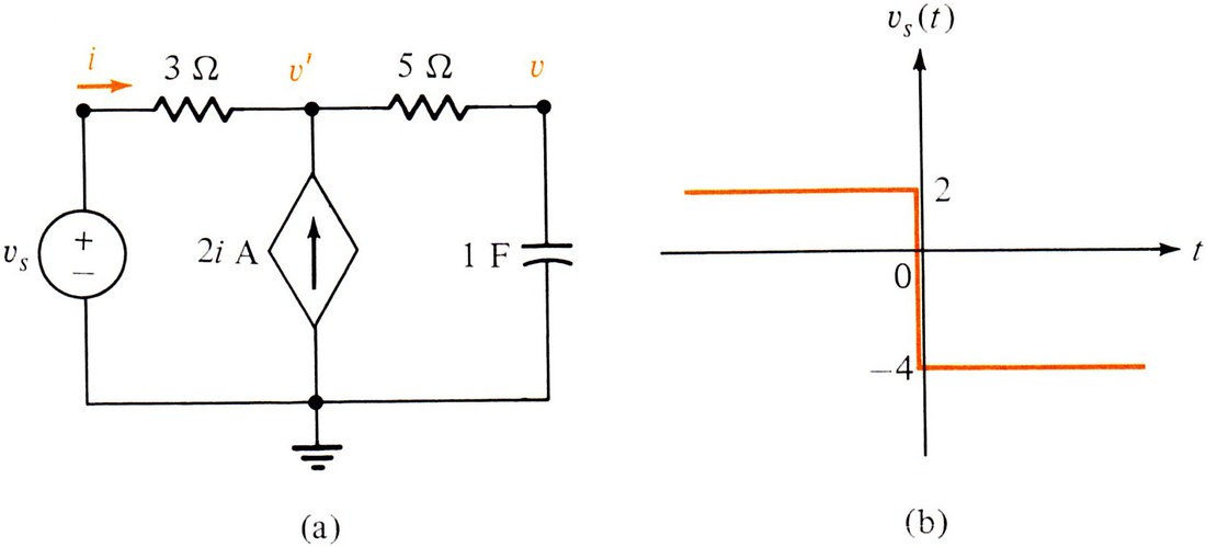
This problem requires two intervals. In the first interval, a DC analysis of the circuit with a source of 2 V gives us the voltage in the capacitor.
s\dc("e,1,0,2:r3,1,2,3:r5,2,3,5:c,3,0,1:j,0,2,2ir3"):vc2
This is the initial condition for the capacitor in the second interval, which we analyze using TR and a source value of -4 V.
s\tr("e,1,0,–4:r3,1,2,3:r5,2,3,5:c,3,0,1,2:j,0,2,2ir3"):vcThis is the expression for the voltage drop in the capacitor after t=0.
The only tool
Bo2's Drill Exercise 5.11
For the circuit of Bo2's Example 5.7, change the value of the capacitor to ¼ F. Find vC(t) for the case that the source is vS(t)=1 V for t<0 and 3V for t≥0.
We let Symbulator know that we are only interested in one variable: vc.
s\only("vc")Then we run the simulation for the first interval, just as we did before, but with the new capacitor and source values.
s\dc("e,1,0,1:o,1,2,o:c,2,o,1/4:r2,2,o,2:r1,2,0,1"):vc-2
This is the initial condition for the next interval. Before we run the simulation for the second interval, we let Symbulator know, again, that we are only interested in one variable: vc.
s\only("vc")Then we run the simulation for the second interval, just as we did before, but with the new capacitor and source values.
s\tr("e,1,0,3:o,1,2,o:c,2,o,1/4,–2:r2,2,o,2:r1,2,0,1"):vcBo2's Figure 5.38 (Impulse)
Find the voltage drop and current in the capacitor, given a source of I δ(t) A, where δ(t) is the impulse function and I is a constant.
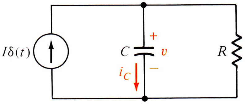
As we mentioned before, impulse sources must be described using the δ(t) nomenclature. To save some typing time, you find it in the menu.
s\tr("j,0,1,i*δ(t):c,1,0,c,0:r,1,0,r")Once the simulation completes, we ask for the variables of interest:
vcicBo2's Drill Exercise 5.13 (Impulse)
For the circuit of Bo2's Example 5.7, find vC(t), iC(t) and vo(t) due to an impulse voltage source of vS(t)= δ(t) (that is to say, a 1V impulse in t=0.)
Nothing new here. Again we use the δ(t) nomenclature for the source.
s\tr("e,1,0,δ(t):o,1,2,o:c,2,o,1/8,0:r2,2,o,2:r1,2,0,1"):{vc,ic,vo}Bo2's Figure 5.39 (Ramp)
Find iL(t) and vL(t) for a circuit that has in parallel a resistor R, an inductor L and a current source with a ramp value I r(t). Initial conditions are zero.
A ramp value I r(t) means a value of I t. We describe this source simply as i*t.
s\tr("j,0,1,i*t:r,1,0,r:l,1,0,l,0"):{il,vl}Bo2's Drill Exercise 5.14 (Ramp)
For the circuit of Bo2's Example 5.7, find vC(t) and iC(t) due to a ramp input voltage of vS(t)= r(t).
Nothing new here. The command below should be clear to you by now.
s\tr("e,1,0,t:o,1,2,o:c,2,o,1/8,0:r2,2,o,2:r1,2,0,1"):{vc,ic}Bo2's Example 5.12 (Exponential)
Assume initial conditions zero. Find iL(t) and vL(t), given that iS(t) = 2 e -4t A.
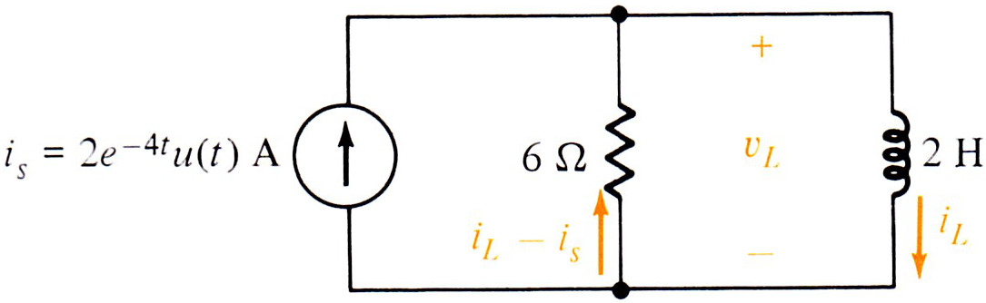
Describe the source as given to you by the problem, using an exponential.
s\tr("j,0,1,2e^(–4t):r,0,1,6:l,1,0,2,0"):{il,vl}Bo2's p265 (Exponential)
Repeat Bo2's Example 5.12 if the current source is now iS(t) = 2 e -3t A.
All we do is change one digit in the circuit description: replace 4 with 3.
s\tr("j,0,1,2e^(–3t):r,0,1,6:l,1,0,2,0"):{il,vl}Bo2's Example 5.13 (Exponential)
Find the voltage drop in the capacitor and the current in the 3 Ω resistor, if the source value is vS(t)=18e-t/2.

s\tr("e,1,0,18e^(–t/2):r3,1,2,3:r5,2,3,5:c,3,0,1,0:j,0,2,2ir3"):{vc,ir3}Bo2's Drill Exercise 5.16 (Exponential)
For the circuit of Bo2's Example 5.7, find vC(t) and iC(t) for the case when the source's value is vS(t)= 2 e -4t. As before, assume initial conditions are zero.
s\tr("e,1,0,2e^(–4t):o,1,2,o:c,2,o,1/8,0:r2,2,o,2:r1,2,0,1"):{vc,ic}Bo2's Example 6.1
Find the current in the inductor i(t) and the voltage drop in the capacitor v(t).

Since we have switches changing in time t=0, this is a two interval problem. The first interval is for t<0. We can analyze the first interval using DC.
s\dc("e,3,0,9:r2,3,1,5:r1,1,0,5:l,1,2,1/2:c,2,0,1/8:r3,2,0,2"):{vc,il}{2,1}These are the initial conditions for the second interval. The second is for t≥0. We can analyze the second interval using TR. We only care about vc and il.
s\only("vc,il"):s\tr("r1,1,0,5:l,1,2,1/2,1:c,2,0,1/8,2"):{vc,il}Notice that the use of the only tool saves approximately 10 seconds here.
The plot tool
Imagine, for example, that in Bo2's Example 6.1 we are asked to plot i(t) and v(t) for times between 0 s and 1.5 s. The first step is to run the plot tool:
s\plot()A window opens, asking you to enter three things: first, a function of time; second, a minimal time; and third, a maximal time. Let's plot vC(t) first. Unless you have deleted the value of the variable vc, you should have the answer to the simulation above stored in it. So enter vc as the function, 0 as the minimal time and 1.5 as the maximal time. Press Enter, and wait a little. The graph of the voltage drop in the capacitor between time 0 and 1.5 seconds should appear in the screen.
Compare it to the graph given by the textbook. Repeat this procedure giving il as the function. Compare the resulting graph to that given by the textbook.

Practice Problems for Lesson 6
Bo2's Drill Exercise 6.1
For the circuit shown, find v(t) and i(t) for t≥0.

Nothing new here. This is a two interval problem, as others seen before. The first interval, for t<0, is analyzed in DC to find the initial conditions.
s\dc("j,0,1,1:r3,1,0,3:r6,1,0,6:l,1,2,1/4:c,2,0,1/3"):{vc,il}{2,0}These conditions are used in the TR analysis of the second interval, for t≥0.
s\only("vc,il"):s\tr("r3,1,0,3:r6,1,0,6:l,1,2,1/4,0:c,2,0,1/3,2")vcilUsing only saves about 13 seconds, or about a third of the calculation time, because only about 8 seconds are used finding the inverse Laplace of the selected answers, instead of 21 seconds finding it for all the answers.
Bo2's Example 6.2
Find i(t) and v(t) for the circuit shown.
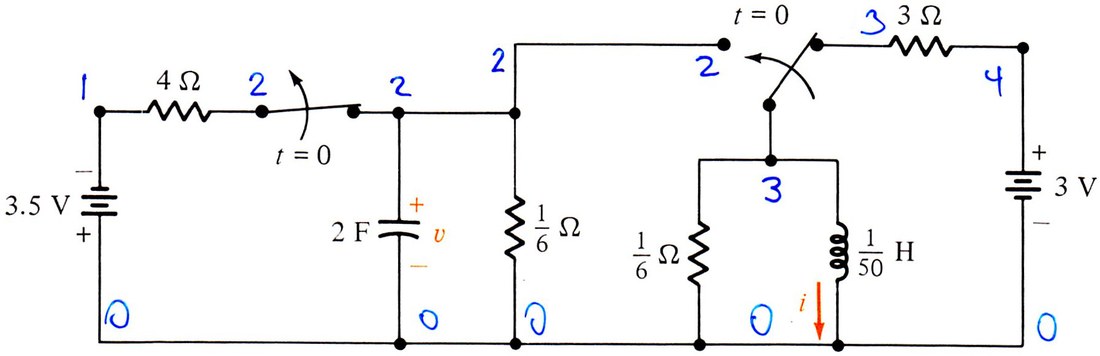
I decided to simulate this using only fractions, not decimals.
So I convert the 3.5V value to its exact fractional equivalent, thus:
exact(3.5)7/2
Because of the switches, this is a two interval problem. The first interval is to be analyzed using DC. Notice that for t<0 the circuit is such that we basically have two separate circuits. We simulate each one of them separately:
s\dc("e1,0,1,7/2:r1,1,2,4:c,2,0,2:r2,2,0,1/6"):vc-7/50
s\dc("r3,3,0,1/6:l,3,0,1/50:r4,3,4,3:e2,4,0,3"):il1
The second interval, for t≥0, is analyzed using TR. I could have described the circuit again from scratch, but out of laziness I copied the descriptions from the DC simulations. To avoid renaming nodes, I simulated the right switch as a short between nodes 2 and 3.
s\only("vc,il"):s\tr("c,1,0,2,–7/50:r,1,0,[1/6,1/6]:l,1,0,1/50,1")vcilThe TR simulation took 30 s in my calculator. These are the right answers.
Bo2's Example 6.3
Find i(t) and v(t) for the circuit shown.
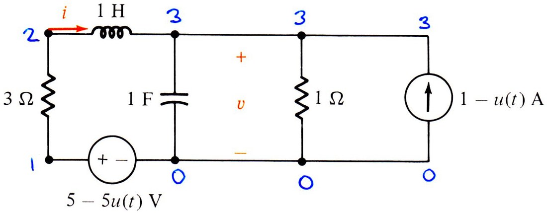
Since the sources change value, this is a two interval problem. For t<0, in DC:
s\dc("e,1,0,5:r3,1,2,3:l,2,3,1:c,3,0,1:r1,3,0,1:j,0,3,1"):{vc,il}{2,1}Using these as initial conditions, now we use TR for t≥0:
s\only("vc,il"):s\tr("r3,0,2,3:l,2,3,1,1:c,3,0,1,2:r1,3,0,1"):{vc,il}Is the textbook wrong?
Anybody who has written a textbook, or read one for that matter, can attest that errors in the problems or the answers come with the territory. (I am sure this book has many.) We are all only human. But errors in an engineering textbook can be very frustrating to a student: confusion and hair-pulling ensue. If you think you have found one in your circuit analysis textbook, Symbulator can help you confirm whether your guess is right.
Below is an example of using Symbulator to confirm an error in a textbook.
Bo2's Drill Exercise 6.4

My copy of Bo2 is second-hand, and this problem had scribbles on it. The previous owner evidently struggled with it and concluded that the inductor had to be ½ H, not the 1 H the schematic says. Symbulator can show he is right and the book wrong. First, solve the circuit as printed, with a 1 H inductor.
s\dc("e,2,0,2:r,1,2,1:l,1,0,1:c,1,0,1/8"):{il,vc}{2,0}s\only("il,vc"):s\tr("r,1,0,1:l,1,0,1,2:c,1,0,1/8,0"):{il,vc}The answer we get doesn't match the answer provided by the book. Now let's repeat the TR simulation using the ½ H value for the inductor:
s\only("il,vc"):s\tr("r,1,0,1:l,1,0,1/2,2:c,1,0,1/8,0"):{il,vc}Now the answer matches the book's. An expert user can reach for the fd gate and the t2s tool, which we have not discussed yet, to find the inductor's value from the book's answer. This is how I found the ½ H myself, working backwards:
s\t2s(–16*t*e^(–4*t)):-16/(s+4)^2
s\t2s((8*t+2)*e^(–4*t))2*(s+8)/(s+4)^2
s\fd("r,1,0,1:l,1,0,l,2:c,1,0,1/8,0"):vc-16*l/(l*s^2+8*l*s+8)
solve(–16/(s+4)^2=–16*l/(l*s^2+8*l*s+8),l)l=1/2
The fd gate and t2s tool are used for frequency domain analysis, and will be discussed separately in a subsequent part of Symbulator's documentation.
Bo2's Drill Exercise 6.5
In the circuit, suppose that vS(t)= 12 – 12 u(t) V. Find i2(t) for t≥0.
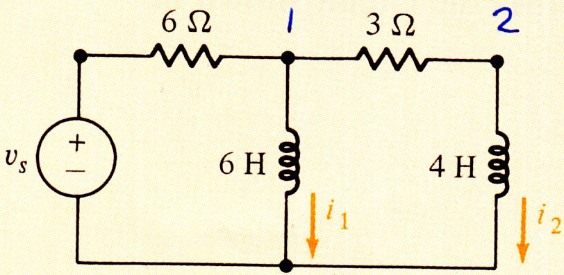
s\dc("e,3,0,12:r6,3,1,6:l1,1,0,6:r3,1,2,3:l2,2,0,4"):{il1,il2}{2,0}s\only("il2"):s\tr("r6,0,1,6:l1,1,0,6,2:r3,1,2,3:l2,2,0,4,0"):il2Bo2's Drill Exercise 6.6 (Op Amp)
In the circuit, suppose that vS(t)= 2 – 2 u(t) V. Find vo(t) for t≥0.

Simulate the first interval in DC to find the initial conditions of the capacitors.
s\dc("e,3,0,2:r1,3,1,1:r2,1,2,2:r3,1,o,2:ca,1,0,1:
cb,2,o,1/4:o,0,2,o"):{vca,vcb}{0,4}Then simulate the second interval in TR, to find the voltage in node o.
s\only("vo"):s\tr("r1,0,1,1:r2,1,2,2:r3,1,o,2:
ca,1,0,1,0:cb,2,o,1/4,4:o,0,2,o"):vo
Bo2's Example 6.5 (Plot)
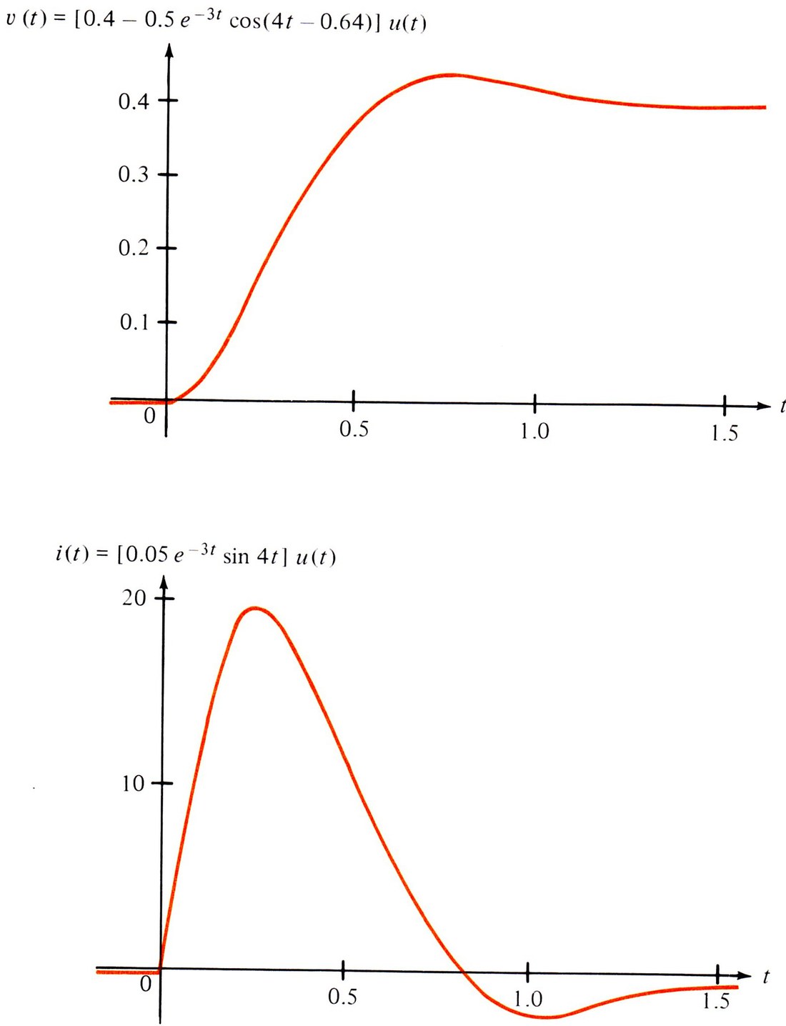
In the circuit, use vS=2/5V, R=12Ω, L=2H and C=1/50F. Find v(t) and i(t), and plot them for time 0<t<1.5 seconds.
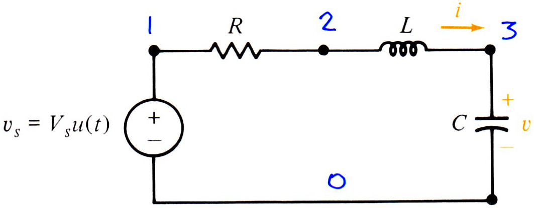
s\only("vc,il"):s\tr("e,1,0,2/5:r,1,2,12:l,2,3,2,0:c,3,0,1/50,0")vc-(2/5)e-3tcos(4t)-(3/10)e-3tsin(4t)+2/5
ilThese are the right answers. To plot them, run the plot tool, thus: s\plot(). Once the plot window opens, enter vc as function, 0 as minimal time and 1.5 as maximal time. Compare to the graph from the book. Repeat the plot for il, and compare that one to the book's graph too.
Bo2's Drill Exercise 6.7
For the circuit in Bo2's Example 6.5, use vS=3V, R=5Ω, L=1/2H and C=1/8F. Find v(t) and i(t).
s\only("vc,il"):s\tr("e,1,0,3:r,1,2,5:l,2,3,1/2,0:c,3,0,1/8,0"):{vc,il}Bo2's Drill Exercise 6.8 (Ramp)
For the circuit in Bo2's Drill Exercise 6.7, find the voltage drop in the capacitor v(t) if the source has a value vS(t) = 3 r(t).
s\only("vc"):s\tr("e,1,0,3t:r,1,2,5:l,2,3,1/2,0:c,3,0,1/8,0"):vcBo2's Example 6.6 (Plot)
For the circuit, plot the voltage drop in the inductor for 0 < t < 5ms.

First, find the initial conditions for t<0 by running a DC simulation.
s\dc("e,1,0,12:r,1,2,3:l,2,3,1:c,3,0,1'µ:s,3,0"):{il,vc}{4,0}Then, find the vl for t≥0 by running a TR simulation.
s\only("vl"):s\tr("e,1,0,12.:r,1,2,3:l,2,3,1,4:c,3,0,1'µ,0")Finally, run s\plot() and enter vl as function, 0 as minimal time and 0.005 as maximal time. In the resulting plot you will see something outstanding: around t = 1.57 ms, the voltage drop across the inductor is 3991 volts!
Bo2's Drill Exercise 6.9
For the circuit, R=1Ω, L=2H, C=1/2F and iS(t)=u(t). Find i(t) and v(t).

s\only("il,vc"):s\tr("j,0,1,1:r,1,0,1:l,1,0,2,0:c,1,0,1/2,0"):{il,vc}Bo2's Figure 6.23 (Op Amp)
For the circuit, find vo(t) if vS(t) = u(t).

s\only("vo"):s\tr("e,3,0,1:r1,3,1,1:r2,1,2,1:
ca,2,0,1/5,0:cb,1,o,1,0:o,2,o,o"):voBo2's Drill Exercise 6.10 (Op Amp)
In the previous circuit, change the capacitor's value from 1/5 F to 25/16 F. Find vo(t) if vS(t) = 3 u(t).
s\only("vo"):s\tr("e,3,0,3:r1,3,1,1:r2,1,2,1:
ca,2,0,25/16,0:cb,1,o,1,0:o,2,o,o"):vo-4e-2t/5+e-8t/5+3
Bo2's Drill Exercise 6.11 (p307)
For the circuit, suppose that R1 = R2 = 1Ω, L = 1H, C = 1F and vS(t)= 2e-2t u(t). Find i(t) if all initial conditions are zero.

s\only("il"):s\tr("e,3,0,2e^(–2t):r2,3,2,1:r1,2,1,1:c,2,0,1,0:l,1,0,1,0"):il-(et cos(t)-et sin(t)-1) e-2t
A more complex problem
The circuit comes from the circuits analysis class of Professor Eliane Boulet de Cabrera, from Universidad Tecnologica de Panama. Find v1 and v.

Because of the switches, this is a two interval problem. The first is run in DC.
s\dc("e,3,0,18:r8,3,1,8:ca,1,0,1/6:r12,1,0,12:
r18,1,2,18:r6,2,0,6:cb,2,0,1/3"):{vca,vcb}{9,9/4}These serve as initial conditions for the second interval, which is run in TR. Since we only want v1 and v2, it pays off to let Symbulator know this:
s\only("v1,v2"):s\tr("ca,1,0,1/6,9:r12,1,0,12:r18,1,2,18:r6,2,0,6:
cb,2,0,1/3,9/4:j,0,2,10e^(–t)sin(2t+30°)")Be patient. This took 78 seconds in my calculator, including over half a minute just to find the inverse Laplace of the two desired answers.
v1v2These are the correct answers, which explains why Professor Boulet – who made the problem up - is a living legend among circuit students at UTP.
Advanced use of Expert in TR
The expert tool can be very useful in transient analysis. Using it, however, requires some knowledge. Here’s two things you need to know in order to use ex like a boss:
First, when Symbulator solves a problem using TR, it follows these general steps:
- Generate a set of equations and unknowns for the system, in the frequency domain. Any time-dependent source is replaced with a dummy variable.
- Solve these frequency domain equations.
- Replace any dummy variable with the original source value, and convert the answers to the time domain.
Second, when Symbulator solves a problem using the expert tool, it freezes this process halfway between steps 1 and 2, so that you can tinker with the equations and unknowns before they are solved.
In the problems below, you will see that, when we tinker with the equations, we have to do so in the frequency domain.
Bo2's Drill Exercise 4.5 (Expert)
For this circuit, we know that the capacitor’s initial condition is zero, that vs is an unknown step source (i.e. of the form A u(t), where A is a constant value in volts) and that the voltage drop in the capacitor for t>0 is found to be 1-e^(-t/2). Find the voltage drop in the resistor, the current through the capacitor and the value of the source.

This problem is a match made in heaven for the expert tool, because we have one unknown value in the circuit (i.e. the value of the step source) and we have one known answer (i.e. the voltage drop in the capacitor.) So, the game plan here is to run this circuit through Symbulator’s expert mode, add one new equation and one new unknown, and then solve. First, let’s generate the new equation.
A non-expert user would think that the new equation is 1-e^(-t/2)=vc. But you know better. You know that Symbulator solves the equations of TR problems in the frequency domain. So we have to convert this expression from the time domain to the frequency domain. Symbulator has a shortcut to invoke DiffEq’s Laplace Transform to do so: s\t2s.
s\t2s(1-e^(–t/2))=vcWe have our new equation. Copy this equation into the clipboard, since we will want to paste it in the Expert window. Now let’s run the Expert simulation of the circuit. Let’s define the value of the source as a*u(t), since we know it’s a step source; the variable a will serve as the unknown value, for which we will solve in the Expert mode.
s\ex("e,1,0,a*u(t):r,1,2,2:c,2,0,1,0")When prompted, select TR as the desired option. Then you will see the typical Expert prompt. In the equations field, paste the new equation, adding the word and first:
and 1/s-2/(2*s+1)=vcIn the unknown field, add the variable a, preceded by a comma:
,aLet Symbulator solve the equations now. Once it is done, we want to do a quick sanity check. If the system solved correctly, we should see that Symbulator has as voltage drop in the capacitor the expression we already know from the problem statement:
vc1-e-t/2
This is correct, so we proceed to ask for the answers we want:
ic(1/2)e-t/2
vre-t/2
aThese are the correct answers. The value of the step source is 1 volt.
Bo2's Drill Exercise 4.13 (Expert)

This problem is solved just like the one we already saw. First, find the new equation:
vr=s\t2s(e^(–t))Then run the Expert simulation. I decided to use vs as the step value of the source:
s\ex("e,1,0,vs*u(t):r,1,2,1:c,2,0,1,0"):When prompted, select TR. In the equations field, add the new equation you found:
and vr=1/(s+1)In the unknowns field, add the new variable:
,vsLet Symbulator rip. Once it finishes solving, ask for the sanity check:
vre-t
Looks good, so go ahead and ask for the answers:
ire-t
vc1-e-t
vsAin’t that a beauty? Yes, ma’am! Atta boy, Symbulator! Atta boy!
Bo2's 164 (Expert)

This is the same thing as the previous two, so there is no need for commentary.
il=s\t2s(1-e^(–2*t))s\ex("e,1,0,vs*u(t):r,1,2,2:l,2,0,1,0")Choose TR, and add ,vs to the unknowns and the following to the equations
and il=1/s-1/(s+2)And solve. When done, ask for the sanity check:
il1-e-2t
Since that adds up, ask for the answers:
vl2e-2t
vr2-2e-2t
vs2
vl*il2e-4t(e2t-1)
This is the end of the TR section.